Background: I was doing some exploratory work for a potential project looking at intramural investigators at the NIH. Eventually I decided to put it aside for the time being, but here is some cleaned up code that came out of it, along with some basic descriptives.
1 The Big Picture
The NIH is usually known for its funding of biomedical research in universities and other research institutions i.e. its extramural program. However, the NIH also employs its own scientists - this is its intramural research program or IRP. The goal of this post is to see if we can use publicly available data on government employees (more on that in a bit) to learn something about that population.
I’m going to do this in two broad steps:
- Get the names of IRP investigators
- Use the names to link to federal employee data from the Office of Personnel Management (courtesty of Buzzfeed)
2 Scraping Investigator Names
You can find the name of all IRP Principal Investigators (PIs) here, or see a screenshot of the page below.
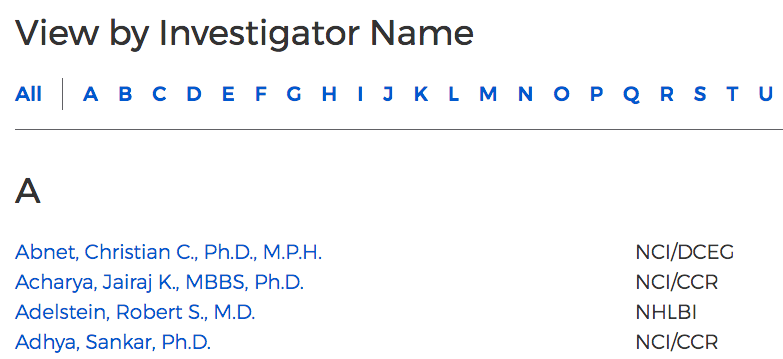
I want to collect all these names without having to copy and paste them. This will help make the analysis reproducible and less prone to error. I’m going to do this with the rvest package, following the steps in the vignette for SelectorGadget.
Selectorgadget is a javascript bookmarklet that allows you to interactively figure out what css selector you need to extract desired components from a page.
What I need to do is go to the page I want to scrape data from and use SelectorGadget to select the elements I want (yellow highlight) and don’t want (red highlight). I end up with this:
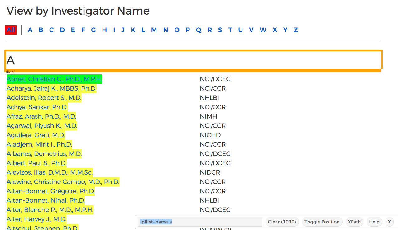
At the bottom of the screenshot, SelectorGadget has determined the right CSS selector needed to extract the names. Now we can move to doing everything in R.
knitr::opts_chunk$set(warning = F, message = F)

library(tidyverse)
## Warning: package 'tibble' was built under R version 3.5.2## Warning: package 'tidyr' was built under R version 3.5.2## Warning: package 'purrr' was built under R version 3.5.2## Warning: package 'dplyr' was built under R version 3.5.2## Warning: package 'stringr' was built under R version 3.5.2library(magrittr)
library(rvest)
html = read_html("https://irp.nih.gov/our-research/principal-investigators/name")
# based on selectorgadget
pi_names_html = html_nodes(html, ".pilist-name a")
pi_names = html_text(pi_names_html)
pi_names[1:5]## [1] "Abnet, Christian C., Ph.D., M.P.H." "Acharya, Jairaj K., MBBS, Ph.D."
## [3] "Adelstein, Robert S., M.D." "Adhya, Sankar, Ph.D."
## [5] "Afraz, Arash, M.D., Ph.D."We now have the PI names as a character vector along with their degrees. To keep things simple, I’m going to extract just their first and last names and ignore the other information.
df = tibble(fullname = pi_names)

# separate name into first, middle, last
df %<>%
  tidyr::extract(fullname,
                 into = c("last_name", "first_name"),
                 regex = "(.+?)\\,\\s(.+?)\\,",
                 remove = FALSE)  %>%
  separate(first_name, into = c("first_name", "middle_name"), sep = "\\s")

df
## # A tibble: 1,062 x 4
## fullname last_name first_name middle_name
## <chr> <chr> <chr> <chr>
## 1 Abnet, Christian C., Ph.D., M.P.H. Abnet Christian C.
## 2 Acharya, Jairaj K., MBBS, Ph.D. Acharya Jairaj K.
## 3 Adelstein, Robert S., M.D. Adelstein Robert S.
## 4 Adhya, Sankar, Ph.D. Adhya Sankar <NA>
## 5 Afraz, Arash, M.D., Ph.D. Afraz Arash <NA>
## 6 Afzali, Behdad (Ben), M.D., Ph.D. Afzali Behdad (Ben)
## 7 Aguilera, Greti, M.D. Aguilera Greti <NA>
## 8 Aladjem, Mirit I., Ph.D. Aladjem Mirit I.
## 9 Albanes, Demetrius, M.D. Albanes Demetrius <NA>
## 10 Albert, Paul S., Ph.D. Albert Paul S.
## # … with 1,052 more rows2.1 Clean names
Below is some code for standardizing the names. I do three things:
- convert to lower case
- replace accented characters with plain ones (e.g. é to e)
- replace non-letters with spaces (e.g. O’Neill to oneill)
# Lower case
df %<>% mutate_at(vars(last_name:middle_name), str_to_lower)

# Replace accents with plain letters
accent_dictionary =
  list('Š'='S', 'š'='s', 'Ž'='Z', 'ž'='z', 'À'='A', 'Á'='A', 'Â'='A', 'Ã'='A', 'Ä'='A', 'Å'='A', 'Æ'='A', 'Ç'='C', 'È'='E', 'É'='E',
       'Ê'='E', 'Ë'='E', 'Ì'='I', 'Í'='I', 'Î'='I', 'Ï'='I', 'Ñ'='N', 'Ò'='O', 'Ó'='O', 'Ô'='O', 'Õ'='O', 'Ö'='O', 'Ø'='O', 'Ù'='U',
       'Ú'='U', 'Û'='U', 'Ü'='U', 'Ý'='Y', 'Þ'='B', 'ß'='Ss', 'à'='a', 'á'='a', 'â'='a', 'ã'='a', 'ä'='a', 'å'='a', 'æ'='a', 'ç'='c',
       'è'='e', 'é'='e', 'ê'='e', 'ë'='e', 'ì'='i', 'í'='i', 'î'='i', 'ï'='i', 'ð'='o', 'ñ'='n', 'ò'='o', 'ó'='o', 'ô'='o', 'õ'='o',
       'ö'='o', 'ø'='o', 'ù'='u', 'ú'='u', 'û'='u', 'ü'='u', 'ý'='y', 'ý'='y', 'þ'='b', 'ÿ'='y')

df %<>%
  mutate(first_name =
           chartr(paste(names(accent_dictionary), collapse = ''),
                  paste(accent_dictionary, collapse = ''), first_name),
         last_name =
           chartr(paste(names(accent_dictionary), collapse = ''),
                     paste(accent_dictionary, collapse = ''), last_name))

# Replace non-letters
df %<>% mutate(first_name = str_replace_all(first_name, "[^a-z]", ""),
               last_name = str_replace_all(last_name, "[^a-z]", ""))
3 OPM data
Now that we have the names of the IRP PIs, let’s see if we can identify them in this awesome dataset that Buzzfeed put online for public use.
The dataset contains hundreds of millions of rows and stretches all the way back to 1973. It provides salary, title, and demographic details about millions of U.S. government employees, as well as their migrations into, out of, and through the federal bureaucracy. In many cases, the data also contains employees’ names.
Thank you, Buzzfeed!
I have the data stored on an external hard drive, so for this part of the code you’ll have to change the file path to wherever you’ve downloaded the data.
# Where you've stored the Buzzfeed data after downloading it
your_root = "/Volumes/research_data"

path = file.path(your_root, "opm-federal-employment-data/data",
       "2016-12-to-2017-03/non-dod/status", "Non-DoD FOIA 2017-04762 201703.txt")

opm2017 = read_delim(path,
                     col_types = cols(),
                     delim = ";",
                     na = c("", "NA", "*", ".", "############"),
                     n_max = Inf)

# install.packages("janitor")
opm2017 %<>%
  janitor::clean_names() %>% # clean column names
  rename(subagency = sub_agency)

opm2017
## # A tibble: 1,355,327 x 19
## last_name first_name file_date agency subagency state age_range ysd_range
## <chr> <chr> <dbl> <chr> <chr> <chr> <chr> <chr>
## 1 NAME WIT… NAME WITH… 201703 TR-DE… TR93-INT… REDA… 60-64 30 - 34 …
## 2 NAME WIT… NAME WITH… 201703 TR-DE… TR93-INT… REDA… 60-64 35 - 39 …
## 3 NAME WIT… NAME WITH… 201703 TR-DE… TR93-INT… REDA… 60-64 40 - 44 …
## 4 NAME WIT… NAME WITH… 201703 TR-DE… TR93-INT… REDA… 60-64 25 - 29 …
## 5 NAME WIT… NAME WITH… 201703 TR-DE… TR93-INT… 11-D… 35-39 10 - 14 …
## 6 HESS KEVIN 201703 VA-DE… VALA-VET… 41-O… 50-54 25 - 29 …
## 7 KELLER STEVEN 201703 VA-DE… VALA-VET… 47-T… 50-54 5 - 9 ye…
## 8 SAPP JAMES 201703 HE-DE… HE35-AGE… 13-G… 50-54 25 - 29 …
## 9 NAME WIT… NAME WITH… 201703 HS-DE… HSBB-IMM… REDA… 50-54 25 - 29 …
## 10 NAME WIT… NAME WITH… 201703 HS-DE… HSBB-IMM… REDA… 50-54 Unspecif…
## # … with 1,355,317 more rows, and 11 more variables: education_level <chr>,
## # pay_plan <chr>, grade <chr>, los_level <chr>, occupation <chr>,
## # patco <chr>, adjusted_basic_pay <dbl>, supervisory_status <chr>, toa <chr>,
## # work_schedule <chr>, nsftp_indicator <chr>I perform the same operations for cleaning names. I also filter the employees belonging to the NIH using the subagency code “HE38”.
# NIH employees only
opm2017 %<>% filter(str_detect(subagency, "HE38"))

# clean names
opm2017 %<>%
  mutate_at(vars(last_name, first_name), str_to_lower) %>%  # set names to lower case
  mutate(first_name = str_replace_all(first_name, "[^a-z]", ""),
         last_name = str_replace_all(last_name, "[^a-z]", "")) %>%
  # replace non-letters with space
  mutate(first_name =
           chartr(paste(names(accent_dictionary), collapse = ''),
                  paste(accent_dictionary, collapse = ''), first_name),
         last_name =
           chartr(paste(names(accent_dictionary), collapse = ''),
                  paste(accent_dictionary, collapse = ''), last_name))
3.1 Linking PI names to OPM payroll data
I’m going to implement a simple matching rule: unique matches on first and last names.
# Give IDs to track duplicates
df %<>%
  mutate(id = row_number()) %>%
  select(id, everything())

opm2017 %<>%
  mutate(opm_id = row_number()) %>%
  select(opm_id, everything())

pi_opm = df %>%
  select(id, last_name, first_name) %>%
  inner_join(opm2017, by = c("last_name", "first_name"))

pi_opm %<>%
  group_by(id) %>%
  mutate(x = n() > 1) %>% # duplicate from dataframe of scraped names
  group_by(opm_id) %>%
  mutate(y = n() > 1) %>% # duplicate from OPM data
  ungroup() %>%
  filter(!x, !y)
We had 1062 names and managed to match 887 of them. We could maybe do better but for such a simple “algorithm” I’m happy enough.
4 What can we learn about the intramural program?
It’s a good idea to take a peek at the data with the wonderful skimr package, even if we will plot some of the variables again later, but this post is getting long so I won’t print the results of that. Age and years of service are reported in 5-year bins, so to I’ve converted them into numeric values based on the lower end of the bin.
pi_opm %<>%
  mutate(age = parse_number(age_range),
         yrs_since_degree = parse_number(ysd_range))

# skimr::skim(pi_opm)
4.1 Aging of the scientifc workforce
A prominent question about the scientific research workforce these days is whether it is aging (yes) and the implications of the aging phenomenon for scientific research.
library(hrbrthemes)
theme_set(theme_ipsum(base_size = 18, axis_title_size = 16))
theme_update(axis.text = element_text(size = 16))

pi_opm %>%
  ggplot(aes(age)) +
  geom_bar() +
  theme_ipsum(grid = "Y", base_size = 18, axis_title_size = 16) +
  labs(y = "Count",
       x = "Age (5-year bin)",
       title = "Intramural investigators seem old")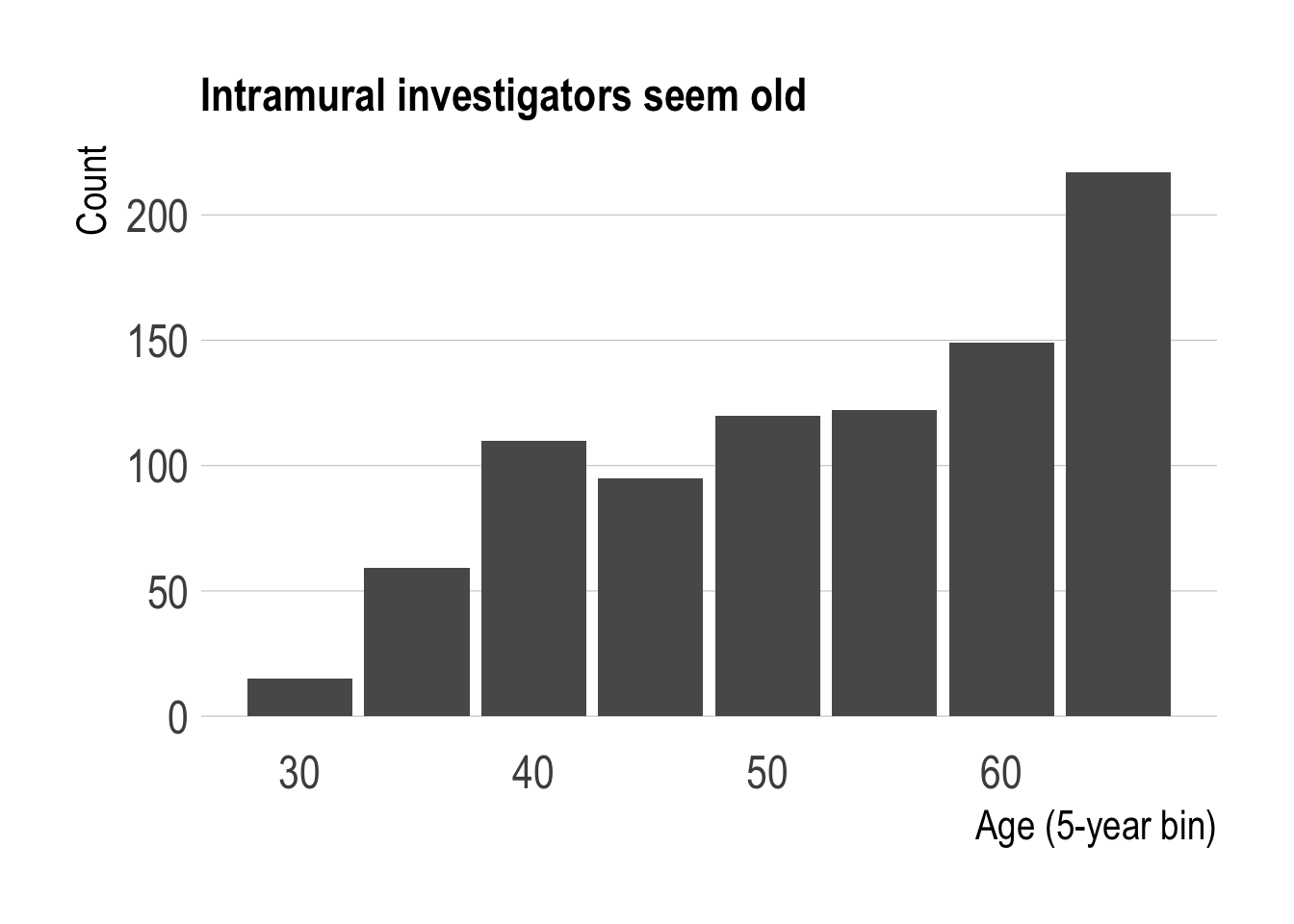
The distribution of the intramural PIs is older than I’d have guessed. Strikingly, PIs older than 65 make up the largest share of the population. It’d be interesting to see how this distribution has changed over time. While this may be related to the general aging phenomenon, research funding or hiring policies could also have an effect.
4.2 How much do scientists earn?
pi_opm %>%
  ggplot(aes(adjusted_basic_pay)) +
geom_histogram() 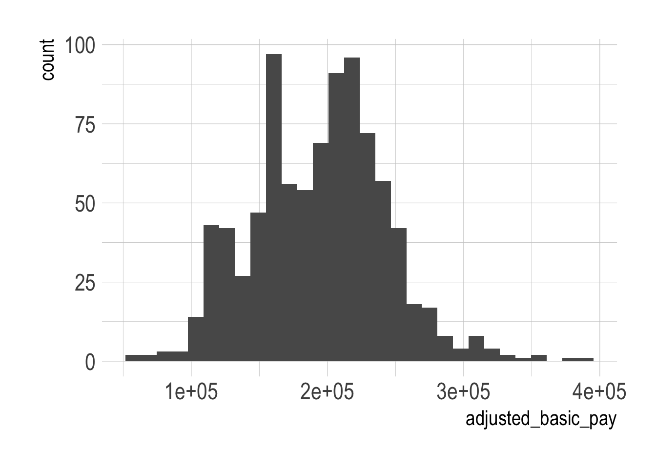
Not a bad living, but there also seems to be a fairly wide range. Some of this might be down to experience, which we can check using years since degree as a proxy.
pi_opm %>%
  ggplot(aes(yrs_since_degree, adjusted_basic_pay)) +
  geom_boxplot(aes(group = yrs_since_degree),
               alpha = 1/2, outlier.shape = NA, size = 1.1) +
  geom_jitter(alpha = 1/3)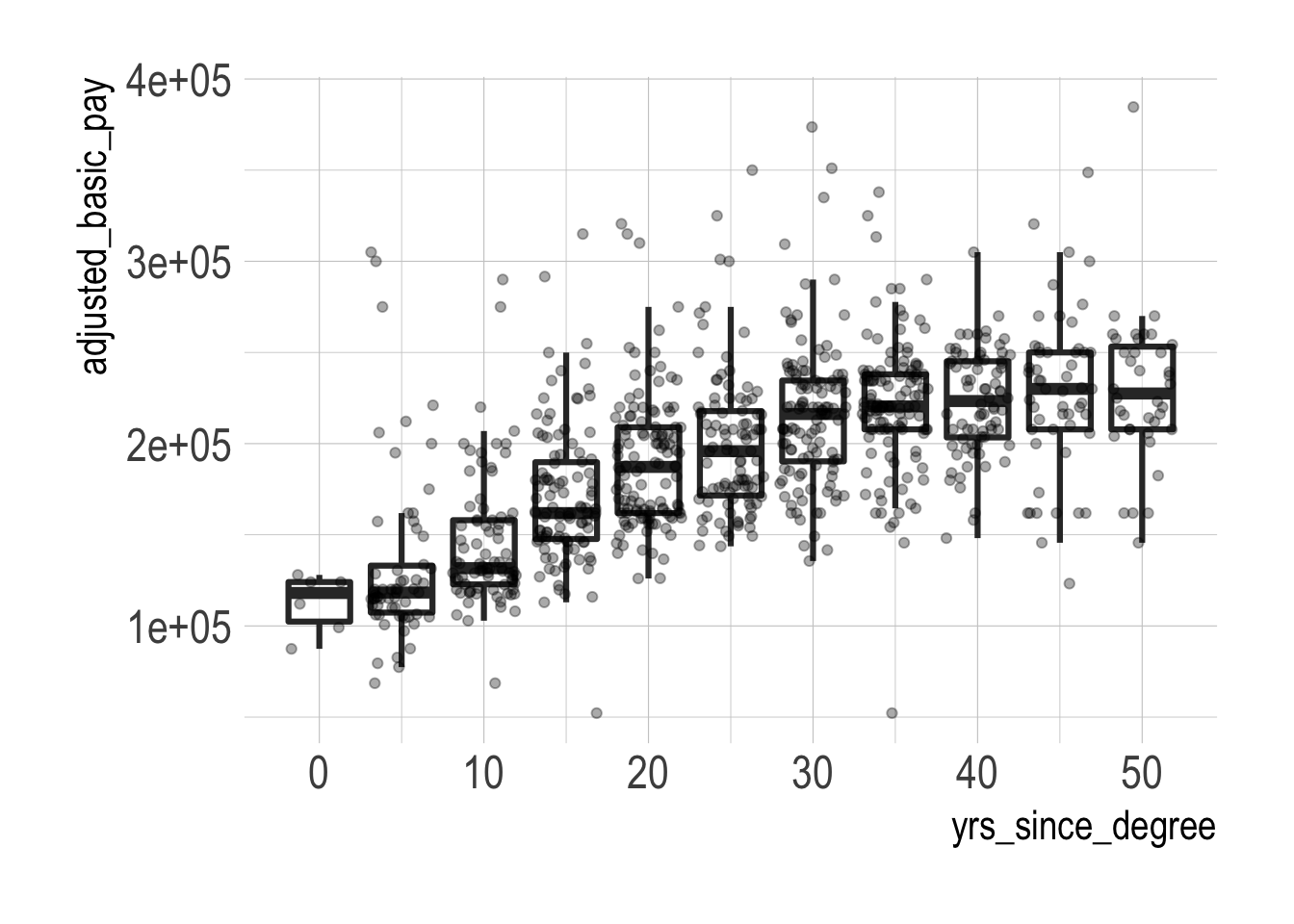
Salary seems to generally increase with years since degree, but there is a fair amount of spread within each yrs_since_degree bin. The median salary also starts to stagnate from the 30-34 bin onwards.
4.3 Gender representation in the intramural program
The actual demographics of the intramural program are available online. The number of female tenured researchers (Senior Investigators) is low at 23%, and increases somewhat as you go to more junior appointments.1
Since gender isn’t available in the OPM data, I’ll use Genni to predict gender based on first name and birth year.
genni = read_tsv(here::here("../Genni/ssnnamesdata.out"),
                 col_types = cols_only(name = "c", `2008` = "c"))

genni %<>%
  rename(probs = `2008`) %>%
  tidyr::separate(probs,
                  into = c("a", "b", "pfem", "d"),
                  sep = "\\|",
                  convert = TRUE) %>%
  select(name, pfem) %>%
  mutate(name = str_to_lower(name))

pi_opm %<>% left_join(genni, by = c("first_name" = "name"))

nafem = pi_opm %>% filter(is.na(pfem)) %>% nrow() # number names without prediction
There are 92 persons whose first names do not appear in Genni. I’ll impose an arbitrary threshold that we have to be at least 75% sure to classify someone as female or male.
pi_opm_fem = pi_opm %>%
  filter(pfem >= 0.75 | pfem <= 0.25) %>%
  mutate(female = pfem >= 0.75)

pi_opm_fem %>%
  count(female) %>%
  mutate(percent = n/sum(n) * 100)
## # A tibble: 2 x 3
## female n percent
## <lgl> <int> <dbl>
## 1 FALSE 560 73.0
## 2 TRUE 207 27.04.3.1 Gender salary differences
pi_opm_fem %>%
  ggplot(aes(adjusted_basic_pay)) +
  geom_density(aes(fill = female), position = "identity", alpha = 0.5) +
  labs(title = "Men tend to earn more")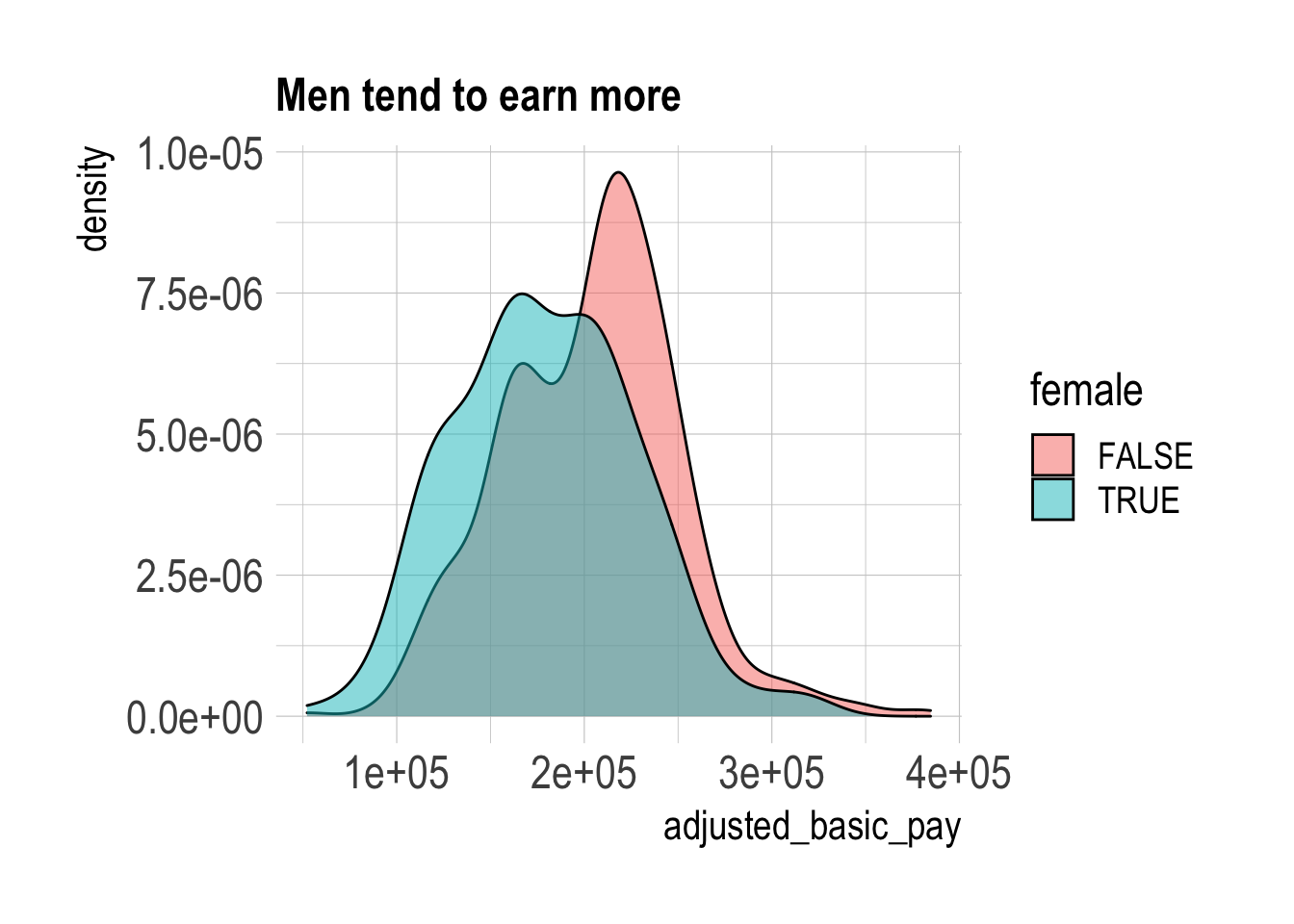
A direct comparison shows that male PIs tend to earn more than female PIs. This isn’t entirely surprising since we know from the IRP website that there are many more men than women in senior appointments, so what happens if we try to “control for” seniority? I’ll run a simple linear regression with controls for the years since degree bins.
mod = lm(log(adjusted_basic_pay) ~ female + factor(yrs_since_degree),
         data = pi_opm_fem)

modgap = mod %>%
  broom::tidy(conf.int = TRUE) %>%
  filter(term == "femaleTRUE") %>%
  mutate(x = "With Controls")

gap = lm(log(adjusted_basic_pay) ~ female, data = pi_opm_fem) %>%
  broom::tidy(conf.int = TRUE) %>%
  filter(term == "femaleTRUE") %>%
  mutate(x = "No Controls") %>%
  bind_rows(modgap)

ggplot(gap, aes(x, abs(estimate))) +
  geom_col() +
  geom_errorbar(aes(ymin = abs(conf.low), ymax = abs(conf.high)), width = 0.2) +
  coord_flip() +
  labs(title = str_wrap("Gender gap remains after accounting for experience", 30),
       x = "Model",
       y = "Log points")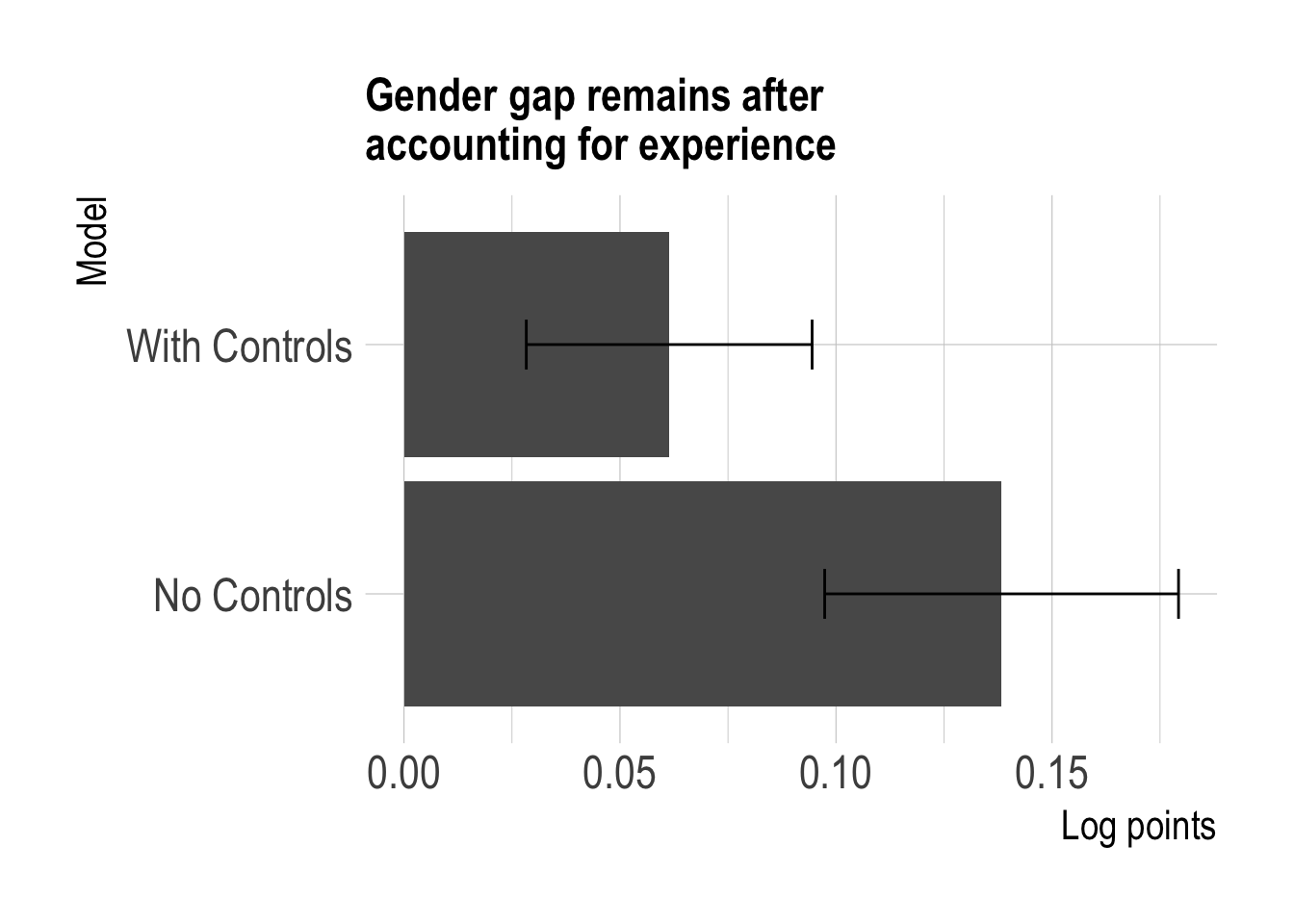
The gap has shrunk by more than half but still remains at about 5-6 percentage points.
Two big caveats here:
- We’re missing a whole lot of information (e.g. productivity, perhaps measured by publication record)
- Even if we did have that information, we should be cautious about how we interpret the gender coefficient
Google, translated: If you control for all the ways we discriminate against women, there's no male-female wage gap. https://t.co/fjVHuJkQDp pic.twitter.com/cew6qpCtUe
— Justin Wolfers (@JustinWolfers) September 14, 2017